Scientific Paper / Artículo Científico
		https://doi.org/10.17163/ings.n36.2026.02
		pISSN: 1390-650X / eISSN: 1390-860X
COMPARATIVE FRAMEWORK FOR ELECTRICITY DEMAND FORECASTING USING MACHINE LEARNING AND ROLLING TEMPORAL VALIDATION
MARCO COMPARATIVO PARA EL PRONÓSTICO DE DEMANDA ELÉCTRICA CON MACHINE LEARNING Y VALIDACIÓN TEMPORAL RODANTE

Juan Carlos Castillo^1,∗ , Jessica N. Castillo¹ , Gabriel Pesántez² , Wilian Guamán²

Received: 15-11-2025, Received after review: 26-01-2026, Accepted: 21-04-2026, Published: 01-07-2026

Abstract	Resumen
Accurate load forecasting is essential for power system planning and operation, particularly under pronounced temporal variability and temporal drift. This study presents a reproducible comparative framework for machine learning models based on rollingorigin expanding validation, multihorizon evaluation, and an operational relative tolerance metric denoted as %Tol. Four representative models are evaluated: EvoXGB, a sequential residual XGBoost ensemble; XGB; TabNet; and FT-Transformer. These models are applied to hourly active power forecasting in distribution substations within an Ecuadorian power system. To ensure a fair comparison when models exhibit differences in prediction coverage or temporal misalignment, the framework incorporates an explicit comparability audit based on temporal alignment and a common evaluation mask denoted as COMMONMASK, complemented the longest common contiguous block for the zoomed time-series visualization. For the representative substation, with metrics computed on the common set, XGB achieves the best performance, with R^2= 0.993 for the short horizon and R^2 = 0.983 for the medium horizon, and RMSE values of 21.16 and 30.84 kW, respectively. EvoXGB remains competitive, whereas TabNet and FT-Transformer exhibit greater degradation in the medium horizon. The 90/10 holdout verification shows the expected performance decline associated with temporal drift while preserving the comparative ranking. Overall, the proposed framework provides a traceable benchmark for substation load forecasting and supports future extensions toward adaptive and hybrid forecasting approaches.	La precisión en el pronóstico de la demanda eléctrica es un elemento central para la planificación y operación de los sistemas de potencia, en particular ante la variabilidad temporal de la carga y la presencia de deriva temporal. En este trabajo se desarrolla un marco comparativo reproducible de modelos de machine learning con validación temporal rodante (rolling-origin expanding), análisis multihorizonte y una métrica operativa de tolerancia relativa (%Tol). Se evalúan cuatro modelos representativos: EvoXGB (ensamble secuencial de XGBoost sobre residuales), XGB, TabNet y FT-Transformer, aplicados al pronóstico horario de potencia activa en subestaciones de distribución de un sistema eléctrico ecuatoriano. Para asegurar la comparabilidad cuando existen diferencias de cobertura o desalineación temporal entre predicciones, se incorpora una auditoría explícita basada en alineación y un conjunto común de evaluación (COMMONMASK), complementada con un bloque contiguo común para la figura de zoom. En la subestación representativa (con métricas sobre el conjunto común), XGB logra el mejor desempeño, con R^2 = 0.993 (corto) y 0.983 (mediano), y un RMSE de 21.16 y 30.84 kW, respectivamente. EvoXGB se mantiene competitivo, mientras que TabNet y FTTransformer muestran mayor degradación en el horizonte mediano. En la verificación de holdout (90/10) se observa la caída esperada por deriva temporal, preservándose el orden comparativo. El marco propuesto entrega una base trazable para comparar modelos en series reales de subestaciones y para extender el análisis hacia esquemas híbridos y adaptativos.
Keywords: load forecasting, machine learning, XGBoost, TabNet, FT-Transformer, rolling temporal validation	Palabras clave: pronóstico de carga, machine learning, XGBoost, TabNet, FT-Transformer, validación temporal rodante.

^1,∗Universidad Técnica de Cotopaxi, Facultad de Ciencias de la Ingeniería y Aplicadas, Ecuador.

Corresponding author ✉: juan.castillo2321@utc.edu.ec.

²Escuela Superior Politécnica de Chimborazo (ESPOCH), GITEA, Riobamba, Ecuador.

Suggested citation: J. C. Castillo, J. N. Castillo, G. Pesántez and W. Guamán. “Comparative framework for electricity demand forecasting using machine learning and rolling temporal validation,” Ingenius, Revista de Ciencia y Tecnología, N.◦ 36, pp. 19-28, 2026, doi: https://doi.org/10.17163/ings.n36.2026.02.

1. Introduction The sustained growth in energy demand and the increasing integration of intermittent renewable sources have made load forecasting a strategic component of power system planning and operation, Accurate forecasting across different time horizons is essential for substation scheduling, resource allocation, and efficient grid management under conditions characterized by seasonality, nonlinear behavior, and regime changes [1, 2], [3–5]. Among contemporary approaches, gradient boosting algorithms, particularly XGBoost, have become widely established due to their robustness and ability to model nonlinear relationships in high-dimensional tabular data [6–9]. However, their performance depends on careful hyperparameter tuning, which is often computationally demanding and sensitive to the dataset configuration. To mitigate this limitation, optimized variants based on evolutionary algorithms have been proposed, including approaches that combine XGBoost with Differential Evolution or Genetic Algorithms, which have demonstrated improvements in stability and reductions in overfitting [10–12]. In parallel, deep learning models specifically designed for tabular data have emerged. TabNet employs sequential attention mechanisms that provide inherent interpretability [13], whereas FT-Transformer adapts the Transformer architecture through linear feature embeddings and multi-head attention [14, 15]. However, several studies indicate that the superiority of deep networks over tree-based methods is not universal and depends strongly on the size and structure of the dataset [16, 17]. A frequent limitation in the load forecasting literature is the use of static training and testing splits that do not account for temporal non-stationarity. Current methodological guidelines recommend temporal validation schemes based on a rolling-origin expanding windows to evaluate model performance over time and detect operational degradation [18–20]. In addition to global metrics such as MAE, RMSE, and R^2, operational indicators that reflect acceptable error tolerances from a planning perspective, such as the %Tol metric, should also be incorporated [21], [22]. Explicit contrast with standard approaches. Unlike random cross-validation or partitioning schemes that do not preserve order, which can produce optimistic estimates by mixing past and future observations, rolling-origin validation evaluates performance in more realistic forecasting scenarios, in which predictions are made for subsequent periods. In addition, the proposed framework integrates conventional performance metrics and the %Tol metric within an explicit comparability audit when prediction coverage differs across models.

In the Ecuadorian context, previous studies have addressed long-term electricity consumption forecasting using machine learning models [23], as well as power system planning through reinforcement learning [24]. This study develops a comparative framework for hourly active power forecasting in substations, based on rolling-origin temporal validation, the %Tol metric, and a methodological audit to ensure fair comparisons. The specific contributions of this study are as follows: i. A reproducible evaluation framework based on rolling temporal validation and micro-criterion metric aggregation is proposed. ii. Boosting-based and deep tabular architectures are compared across short- and medium-term forecasting horizons under a consistent methodological setting. iii. An explicit comparability audit based on temporal alignment and COMMONMASK is incorporated, together with an operational interpretation through the %Tol metric. 2. Materials and Methods 2.1.Data and Variables This methodology evaluates the stability and accuracy of predictive models for electricity demand forecasting in Ecuadorian substations. Hourly active power time series recorded at nine substations of a distribution network within the national power system were used, with approximately 40,000 hourly observations per substation, spanning a continuous 4.5-year period between 2020 and 2024. The data were obtained from internal historical records of the national electric utility. The target variable was active power in kW, while the predictor variables included: i. calendar attributes namely hour, day of the week, and month; ii. lagged power values from 4 to 24 h; and iii. moving averages over 3, 6, and 24 h. For confidentiality reasons, the substation identifiers were anonymized. Each model was trained independently for each substation. To maintain a compact presentation, the tables and figures detail the results of a representative substation, while the remaining substations are used to confirm the consistency of the findings. Specifically, a substation was considered representative when its performance profile, defined by RMSE and %Tol across both forecasting horizons, was closest to the median of the full set according to the sum of ranks, thereby avoiding the selection of extreme cases.

2.2.Data Preprocessing The series were chronologically ordered, and an initial cleaning procedure was performed to remove extreme or infinite values. Missing values were handled using forward filling within each series; any residual cases were discarded to avoid interpolations that could introduce temporal bias. Subsequently, lagged features and moving averages were generated, and the first 24 observations were removed to prevent edge inconsistencies. In each iteration of the validation process, the explanatory variables were scaled using RobustScaler, which was fitted exclusively on the training data of the corresponding window and then applied to the test set to avoid data leakage. For TabNet, the same feature set was retained, with normalization performed internally within the model. 2.3.Prediction Models Analyzed Four representative models were evaluated: A_EvoXGB: a four-stage sequential ensemble based on XGBoost, in which each component trains trees on the residuals of the preceding model. The final prediction is obtained as the sum of the partial outputs, with the aim of reducing systematic error. B_XGB: a standard implementation of XGBoost, used as a robust baseline. C_TabNet: a tabular network with sequential attention [13], configured with nd = na = 32, four decision steps, and early stopping. D_FT-Transformer (D_FTT): a tabular Transformer based on feature embeddings and multihead attention [14, 15], configured with three encoder blocks, a token dimension of 192, and four attention heads. 2.4.Hyperparameter Tuning The most influential hyperparameters were tuned through bounded pilot experiments centered on configurations recommended for medium-sized tabular datasets. The final selection prioritized temporal stability over marginal local improvements while maintaining a comparable training budget. 2.5.Rolling-Origin Temporal Validation Scheme Rolling-origin expanding validation was applied. Two forecasting horizons were considered:

· Short horizon: test window of 168 h, step of 24 h, and purge of 24 h. · Medium horizon: test window of 720 h, step of 72 h, and purge of 72 h. In each iteration, the training set included all observations prior to the start of the test window, excluding the purge period, with a minimum of 1500 observations. The metrics were aggregated using a micro-criterion, jointly considering all predictions generated by each model–horizon combination. 2.6.Temporal Alignment and Common Evaluation Set (COMMONMASK) In practice, different models may produce predictions with unequal coverage, for example, due to partial window execution, or with temporal misalignment caused by offsets related to lag construction or the forecast anchoring point. To avoid biased comparisons, the following audit procedure was applied: · Alignment: a shift of -24 h was applied to the predictions of B_XGB to homogenize the temporal anchoring of the test index with that of the other models. This correction was verified by matching the start of the test segment. · COMMON ALL: the intersection of indices for which all four models provided finite predictions was defined, and the metrics, namely MAE, RMSE, R^2 and %Tol, were computed on this set. · COMMON CONTIG: for the zoom figure, the longest contiguous common block was selected. From this block, a representative 168 h segment was presented to facilitate visual comparison without discontinuities. Note on coverage and non-imputation. When a model presents partial coverage, for example, due to computational constraints or incomplete execution during rolling validation, the common set may be substantially reduced. To avoid bias, missing predictions were neither imputed nor interpolated. Instead, coverage, reported in Table 2, and the size of the common set, reported in Table 3, are explicitly documented. Performance interpretation is therefore limited to the comparable segment. In addition, a 90/10 holdout verification and an aggregated %Tol analysis across nine substations are included to strengthen the conclusions beyond the analysis of a single series.

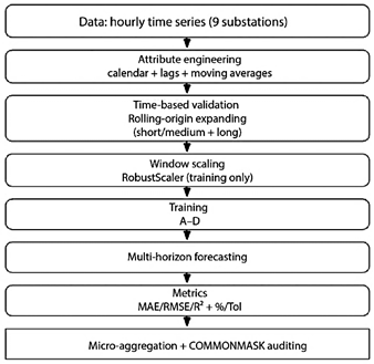
2.7.Summary of the Experimental Pipeline (Scheme)

Figure 1 summarizes the complete sequence of the experimental framework, from data preparation and feature engineering to temporal validation, model training, prediction, and metric aggregation.

Figure 1. Schematic representation of the experimental workflow, including feature extraction, temporal validation, model training, prediction, metric computation, and the comparability audit.

2.8.Independent Validation (90/10 Holdout)

As a complementary verification, each model was retrained using the initial 90% of the data and evaluated on the final 10%, allowing its performance to be assessed outside the temporal recalibration setting.

2.9.Evaluation Metrics

MAE, RMSE, and R² were computed, together with the %Tol metric:

(1)

where δ is the relative tolerance threshold, and ε = 1 kW prevents unstable ratios.

2.10. Reproducibility and Computational Resources

The experiments were conducted in Python 3.11 using XGBoost 2.0, PyTorch 2.3, and PyTorch-TabNet 4.1, with a fixed global seed. Training was performed on an

NVIDIA RTX 3060 GPU (12 GB) with 32 GB of RAM. The scripts and configuration files are available in the GitHub repository [25].

3. Results and Discussion

3.1.Demand Behavior in the Substations

The nine substations analyzed exhibit typical hourly patterns of distribution networks, including nighttime eminima, morning increases, daytime plateaus, and evening peaks, together with weekly seasonality. In the representative substation, active power remains withi na stable operating range, and the observed regim echanges are mainly associated with weekly and seasonal variations, which supports the need for explicit temporal validation.

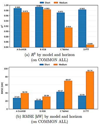
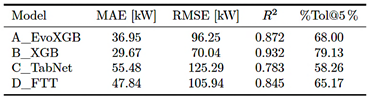
3.2.Global Performance by Model and Horizon

Figure 2 summarizes model performance across models and forecasting horizons under rolling-origin validation. Metrics were computed on COMMON ALL to ensure that all models were evaluated at the same time instants. For this substation, B_XGB achieves the best balance between accuracy and temporal stability across both horizons, while A_EvoXGB remains closely competitive. TabNet and FT-Transformer exhibit greater degradation in the medium-term horizon.

Figure 2. Model performance across forecasting horizons under rolling-origin validation.

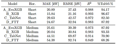
Tabla 1. Performance of the representative substation under micro-aggregation, computed over COMMON ALL: MAE, RMSE, R², and %Tol@5%. (Decimal separator: dot).

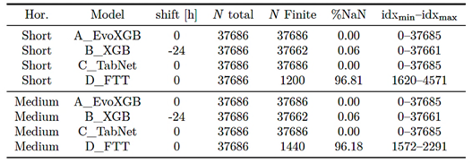
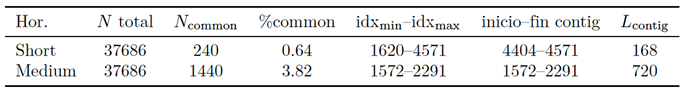
3.3.Comparability Audit: Coverage and COMMONMASK Table 2 reports prediction coverage by model and forecasting horizon, including the total length, number of finite predictions, and percentage of NaN values. Table 3 summarizes the size of the common set (COMMON

ALL) and the longest contiguous common block (COMMON CONTIG), used for the zoom figure. For this substation, the size of COMMON ALL is determined by the model with the lowest coverage (D_FTT); therefore, the audit is explicitly included to ensure transparency.

Table 2. Prediction coverage by model and forecasting horizon for the representative substation.

Table 3. Summary of the common set (COMMONMASK) by forecasting horizon for the representative substation.

In the short horizon, the common set is reduced to 240 h because D_FTT produced predictions over a partial block, and the simultaneous intersection with the other models, after the alignment adjustment of B_XGB, limits the overlap. Therefore, these metrics describe the comparative performance only over this common segment, without imputation. To support the operational conclusions, the analysis also considers (i) the medium horizon, where the overlap is greater (COMMON CONTIG = 720 h in this substation), (ii) the 90/10 holdout verification, and (iii) the aggregated %Tol sensitivity across the nine substations.

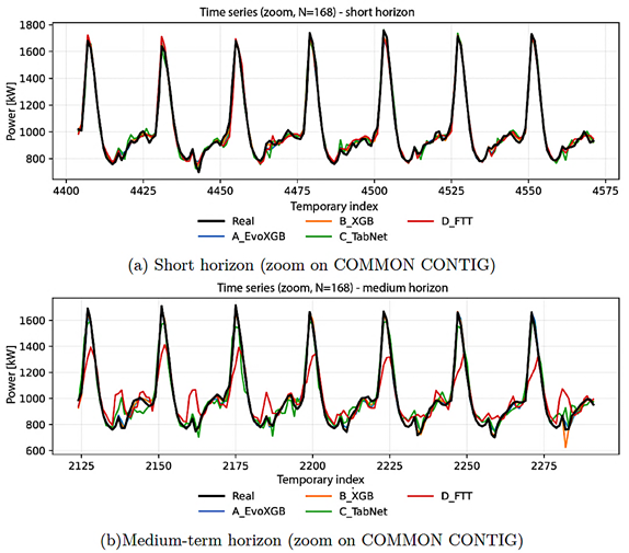
3.4.Temporal Reconstruction of the Load Signal Figure 3 compares the actual series and the model predictions over a representative 168 h segment extracted from the COMMON CONTIG block for both forecasting horizons. The boosting-based models provide a more accurate reconstruction of peaks and valleys. In the medium-term horizon, TabNet and FTTransformer exhibit a degraded fit, consistent with the increase in RMSE and the decrease in R^2.

Figure 3. Actual and predicted series over a representative segment.

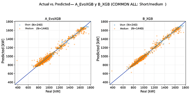
3.5.Relationship Between Observed and Predicted Values Figures 4 and 5 show the relationship between observed and predicted values under rolling-origin validation for both forecasting, evaluated on COMMON ALL. In the

boosting-based models, especially B_XGB, the predictions are more tightly concentrated around the diagonal y = x in both horizons. In C_TabNet and, more notably, D_FTT, dispersion increases in the medium-term horizon, consistent with the increase in RMSE and the reduction in R^2.

Figure 4. Observed vs. predicted values for A_EvoXGB and B_XGB across both forecasting horizons (rolling-origin; COMMON ALL). The line indicates y = x.

Figure 5. Observed vs. predicted values for C_TabNet and D_FTT across both forecasting horizons (rolling-origin; COMMON ALL). The line indicates y = x.

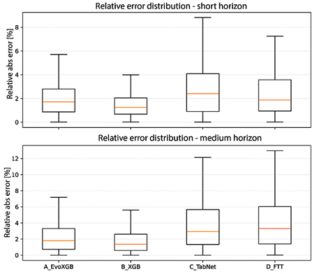
3.6.Distribution of Relative Errors To complement the aggregated metrics and characterize variability, Figure 6 presents the distribution of the

relative absolute error (%). The boosting-based models concentrate errors in lower ranges with shorter tails, while TabNet and D_FTT exhibit greater dispersion, particularly in the medium-term horizon.

Figure 6. Distribution of relative absolute error (%) by model and horizon forecasting horizon under rolling-origin validation.

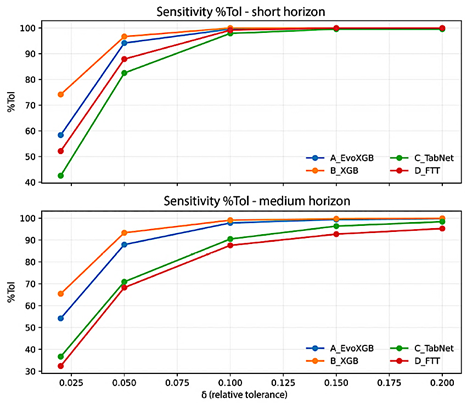
3.7.Operational Metric: %Tol Sensitivity to Threshold δ Figure 7 summarizes the sensitivity of %Tol to different tolerance thresholds. δ was evaluated at 2%, 5%, 10%,

15%, and 20%, aggregating predictions across nine substations. At δ = 5%, the metric clearly distinguishes performance between model families; at δ ≥ 10%, most methods approach 100%, reducing the discriminative capacity of the indicator.

Figure 7. Sensitivity of %Tol to the tolerance threshold δ by model and forecasting horizon (aggregated across the nine substations).

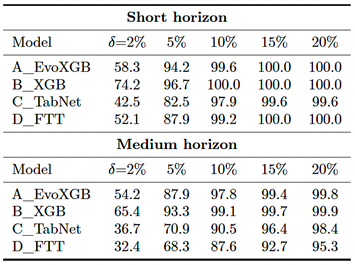
Table 4. Sensitivity of %Tol(δ) by model and forecasting horizon (aggregated across the nine substations). 3.8.Independent Validation (90/10 Holdout) Table 5 shows the expected decrease relative to rolling -origin validation, reflecting temporal drift between evaluation periods. The comparative ranking is preserved, with B_XGB outperforming the other models in this substation. Table 5. Performance under 90/10 holdout validation for the representative substation: MAE, RMSE, R^2,and %Tol@5%.

3.9.General Discussion In the representative substation, tree-based methods maintain the best balance between accuracy and operational interpretability. The alignment audit and COMMONMASK prevent biased comparisons when prediction coverage differs across models or when temporal misalignment is present. TabNet and D_FTT provide an adequate fit in the short-term horizon; however, in the medium-term horizon, they exhibit performance degradation and greater dispersion. Limitations. The data were obtained from a specific system, and the analysis relied on calendar variables, lagged features, and moving averages; therefore, patterns may differ in other contexts or when exogenous variables are incorporated. The representative substation was selected only to provide a clear and compact presentation, while the operational conclusions are strengthened by the aggregated %Tol sensitivity analysis across the nine substations. Finally, when a model presents partial coverage, the common set may be small, as observed in the 240 h short-horizon segment of this substation. Accordingly, the coverage and COMMONMASK audit is explicitly reported, and extrapolation beyond the evaluated common segment is avoided. Future work should incorporate meteorological and renewable generation variables and explore adaptive recalibration schemes and hybrid approaches.

4. Conclusions This study presented a comparative framework of machine learning models applied to hourly electricity demand forecasting in substations, based on rollingorigin temporal validation, multihorizon analysis, and an operational relative tolerance metric. To ensure comparability under differences in prediction coverage and temporal misalignment, an explicit audit using alignment and COMMONMASK (common evaluation mask) was incorporated, with coverage also reported for contextual interpretation. Under rolling-origin validation on COMMON ALL, B_XGB achieved the best performance in the representative substation, followed by A_EvoXGB. TabNet and D_FTT exhibited more pronounced degradation in the medium-term horizon. In the 90/10 holdout validation, the expected performance decline associated with temporal drift was observed, while the relative ranking was preserved. In particular, when the COMMON ALL intersection is small due to partial coverage, as observed in the short horizon of the representative substation, the metrics are interpreted as performance over the strictly comparable segment. Therefore, the conclusions are mainly supported by the medium-term horizon, the holdout validation, and the aggregated %Tol analysis. The proposed framework provides a traceable basis for comparing forecasting approaches and supporting planning and operational decisions. Future work should incorporate exogenous variables, explore adaptiv recalibration, and extend the window-based audit to all models to uniformly characterize temporal stability. Contributor Roles · Juan Carlos Castillo: conceptualization; methodology; data curation; software; formal analysis; research; validation; visualization; project management. · Jessica N. Castillo: methodology; supervision; validation; writing – original draft; writing – revision and editing. · Gabriel Pesántez: methodology; supervision; validation; writing – original draft; writing – revision and editing. · Wilian Guamán: methodology; supervision; validation; writing – original draft; writing – revision and editing.

References [1] T. Hong and S. Fan, “Probabilistic electric load forecasting: A tutorial review,” International Journal of Forecasting, vol. 32, no. 3, pp. 914–938, 2016. [Online]. Available: https://doi.org/10.1016/j.ijforecast.2015.11.011 [2] IEA, “Renewables 2023: Analysis and forecast to 2028,” International Energy Agency, Paris, France, Tech. Rep., 2023, accessed: May 15, 2026. [Online]. Available: https://upsalesiana.ec/ing36ar2r2 [3] M. G. Pinheiro, S. C. Madeira, and A. P. Francisco, “Short-term electricity load forecasting—a systematic approach from system level to secondary substations,” Applied Energy, vol. 332, p. 120493, Feb. 2023. [Online]. Available: https://doi.org/10.1016/j.apenergy.2022.120493 [4] S. Akhtar, S. Shahzad, A. Zaheer, H. S. Ullah, H. Kilic, R. Gono, M. Jasiński, and Z. Leonowicz, “Short-term load forecasting models: A review of challenges, progress, and the road ahead,” Energies, vol. 16, no. 10, p. 4060, May 2023. [Online]. Available: https://doi.org/10.3390/en16104060 [5] F. Rodrigues, C. Cardeira, J. M. F. Calado, and R. Melicio, “Short-term load forecasting of electricity demand for the residential sector based on modelling techniques: A systematic review,” Energies, vol. 16, no. 10, p. 4098, May 2023. [Online]. Available: https://doi.org/10.3390/en16104098 [6] T. Chen and C. Guestrin, “XGBoost: A scalable tree boosting system,” in Proceedings of the 22nd ACM SIGKDD International Conference on Knowledge Discovery and Data Mining, ser. KDD ’16. ACM, Aug. 2016, pp. 785–794. [Online]. Available: https://doi.org/10.1145/2939672.2939785 [7] G. Ke, Q. Meng, T. Finley, T. Wang, W. Chen, W. Ma, Q. Ye, and T.-Y. Liu, “Lightgbm: a highly efficient gradient boosting decision tree,” in Proceedings of the 31st International Conference on Neural Information Processing Systems, ser. NIPS’17. Red Hook, NY, USA: Curran Associates Inc., 2017, p. 3149–3157. [Online]. Available: https://upsalesiana.ec/ing36ar2r4 [8] L. Prokhorenkova, G. Gusev, A. Vorobev, A. V. Dorogush, and A. Gulin, “Catboost: unbiased boosting with categorical features,” in NIPS’18: Proceedings of the 32nd International Conference on Neural Information Processing Systems. arXiv, 2017, pp. 6639–6649. [Online]. Available: https://doi.org/10.48550/arXiv.1706.09516 [9] C. Bentéjac, A. Csörgő, and G. Martínez- Muñoz, “A comparative analysis of gradient boosting algorithms,” Artificial Intelligence Review, vol. 54, no. 3, pp. 1937–1967, Aug. 2020. [Online]. Available: https://doi.org/10.1007/s10462-020-09896-5

[10] Z. Mustaffa and M. H. Sulaiman, “Advanced forecasting of building energy loads with XGBoost and metaheuristic algorithms integration,” Energy Storage and Saving, vol. 4, no. 4, pp. 421–438, Dec. 2025. [Online]. Available: https://doi.org/10.1016/j.enss.2025.03.005 [11] T.-N. Tran and Q.-D. Nguyen, “Research on the influence of genetic algorithm parameters on XGBoost in load forecasting,” Engineering, Technology & Applied Science Research, vol. 14, no. 6, pp. 18 849–18 854, Dec. 2024. [Online]. Available: https://doi.org/10.48084/etasr.8863 [12] B. Liang, W. Qin, and Z. Liao, “A differential evolutionary-based xgboost for solving classification of physical fitness test data of college students,” Mathematics, vol. 13, no. 9, p. 1405, Apr. 2025. [Online]. Available: https://doi.org/10.3390/math13091405 [13] S. Arik and T. Pfister, “TabNet: Attentive interpretable tabular learning,” Proceedings of the AAAI Conference on Artificial Intelligence, vol. 35, no. 8, pp. 6679–6687, May 2021. [Online]. Available: https://doi.org/10.1609/aaai.v35i8.16826 [14] Y. Gorishniy, I. Rubachev, V. Khrulkov, and A. Babenko, “Revisiting deep learning models for tabular data,” in NIPS’21: Proceedings of the 35th International Conference on Neural Information Processing Systems. arXiv, 2021, pp. 18 932–18 943. [Online]. Available: https://doi.org/10.48550/arXiv.2106.11959 [15] V. Borisov, T. Leemann, K. Seßler, J. Haug, M. Pawelczyk, and G. Kasneci, “Deep neural networks and tabular data: A survey,” IEEE Transactions on Neural Networks and Learning Systems, vol. 35, no. 6, pp. 7499–7519, 2024. [Online]. Available: https://doi.org/10.1109/TNNLS.2022.3229161 [16] L. Grinsztajn, E. Oyallon, and G. Varoquaux, “Why do tree-based models still outperform deep learning on tabular data?” in NIPS’22: Proceedings of the 36th International Conference on Neural Information Processing Systems. arXiv, 2022, pp. 507–520. [Online]. Available: https://doi.org/10.48550/arXiv.2207.08815 [17] R. Shwartz-Ziv and A. Armon, “Tabular data: Deep learning is not all you need,” Information Fusion, vol. 81, pp. 84–90, May 2022. [Online]. Available: https://doi.org/10.1016/j.inffus.2021.11.011

[18] V. Cerqueira, L. Torgo, and I. Mozetič, “Evaluating time series forecasting models: an empirical study on performance estimation methods,” Machine Learning, vol. 109, no. 11, pp. 1997–2028, Oct. 2020. [Online]. Available: https://doi.org/10.1007/s10994-020-05910-7 [19] R. J. Hyndman and G. Athanasopoulos, Forecasting: Principles and Practice, 3rd ed. Melbourne, Australia: OTexts, 2021, accessed: May 15, 2026. [Online]. Available: https://upsalesiana.ec/ing36ar2r16 [20] C. Bergmeir and J. M. Benítez, “On the use of cross-validation for time series predictor evaluation,” Information Sciences, vol. 191, pp. 192–213, May 2012. [Online]. Available: https://doi.org/10.1016/j.ins.2011.12.028 [21] M. Q. Raza and A. Khosravi, “A review on artificial intelligence based load demand forecasting techniques for smart grid and buildings,” Renewable and Sustainable Energy Reviews, vol. 50, pp. 1352–1372, Oct. 2015. [Online]. Available: https://doi.org/10.1016/j.rser.2015.04.065 [22] C. Borges, Y. Penya, I. Fernández, J. Prieto, and O. Bretos, “Assessing tolerance-based robust short-term load forecasting in buildings,” Energies, vol. 6, no. 4, pp. 2110–2129, Apr. 2013. [Online]. Available: https://doi.org/10.3390/en6042110 [23] W. Guamán, P. Benalcázar, J. Córdova-García, and M. Torres, Machine Learning-Based Projections of Long-Term Electricity Consumption: The Case Study of Ecuador. Springer Nature Switzerland, 2025, pp. 174–187. [Online]. Available: https://doi.org/10.1007/978-3-031-83432-5_12 [24] G. Pesántez, W. Guamán, J. Córdova, M. Torres, and P. Benalcázar, “Reinforcement learning for efficient power systems planning: A review of operational and expansion strategies,” Energies, vol. 17, no. 9, p. 2167, May 2024. [Online]. Available: https://doi.org/10.3390/en17092167 [25] J. C. Castillo. (2026) Forecasting-rollingenergy. GitHub repository. [Online]. Available: https://upsalesiana.ec/ing36ar2r27